Daniel M. Packer

NOTE: The .xlsx file is available for download; however, the data was prepared and analyzed in JMP Student Edition 18.

NOTE: The .xlsx file contains two worksheets. One of those worksheets is the data dictionary that was provided; I did not create it.

Introduction and Business Understanding: According to Federal Reserve et al. (2005), home equity loans (HELs) are “attractive to consumers” but “all relevant risk factors should be considered when establishing product offerings and underwriting guidelines” before a financial institution underwrites a HEL. The purpose of this study was to perform comparative predictive modeling to determine the best model to use to predict whether a consumer is a good risk for an HEL.

Data Understanding: The raw Equity dataset contained 5,960 records, with one response variable (BAD) and 11 predictor variables. After adjusting for missing values and outliers in the dataset, the dataset was reduced to 3,332 records. From this new dataset, the records were randomly partitioned into training (60%), validation (20%), and test (20%) sets. Next, the modeling type of each column was reviewed, and it was found that BAD needed to be changed from continuous to nominal. Also, the values of 0 and 1 for BAD were recoded as “Good Risk” and “Bad Risk,” respectively (see Figures 2, 3, and 5). The predictors were then reviewed to determine whether any should be excluded from the study, as the explanation of the predictors in the raw dataset were rather vague. The predict CLAGE was defined as “client loan age,” which could be the age of one loan or multiple loans or the age of the client who applied for the loan. Due to the risk of exposure to discrimination of a protected class (age), and due to the vagueness and interpretability of the CLAGE predictor, the CLAGE predictor was excluded from the models.

A feature-engineered BADCLTV ratio was created, where the combined loan to value (CLTV), based on the generally accepted good CLTV ratio of no greater than 80%, was computed for each risk by adding LOAN and MORTDUE and dividing that sum by VALUE, with a cutoff of BADCLTV ≤ 80% coded as 0, meaning good, and a BADCLTV > 80%, coded as 1 meaning bad.

The following predictors were binned by splitting and pruning decision trees in JMP: JOB and YOJ, DEROG, DELINQ, NINQ, CLNO, and DEBTINC. These predictors, and the feature-engineered BADCLTV predictor, were used for the models.

Analysis and Quality of Models: After the data was prepared, decision tree, bootstrap forest, boosted tree, neural network, and boosted neural network models were created, and the validation data was comparatively analyzed based on the sensitivity, specificity, false positive rate, false negative rate, error rate, and AUC (Figure 1); the ROC curve (Figure 2); the lift curve (Figure 3); the misclassification rate (Figure 4); and the cumulative gains curve (Figure 5) of each model.The metrics and outputs of the five models are discussed in the following five subsections.

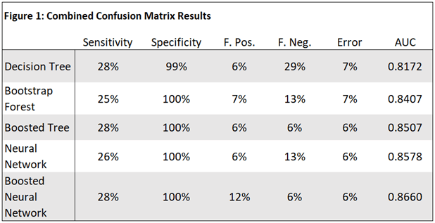
Combined Confusion Matrix: The combined confusion matrix results (Figure 1) show that the sensitivity across all models ranged from 25% to 28%, with the lowest being the bootstrap forest, and that the specificity was 100% for all models but for the decision tree. The boosted tree and the boosted neural network tied for the highest sensitivity and specificity at 28% and 100%, respectively, meaning that both models predicted actual bad risks 29% of the time but good risks 100% of the time. The false positive and false negative rates ranged from 6% to 12% and 6% to 29%, respectively, with the lowest being 6% each for the boosted tree. This means that the boosted tree incorrectly predicted both bad and good risks 6% of the time. The approximate error rates, based on the misclassification rates (Figure 4), ranged from 6% to 7%, with the boosted tree, the neural network, and the boosted neural network models having the lowest error rate of 6%. The area under the curve (AUC) ranged from approximately 81.7% to 86.6%, with the boosted neural network having the greatest AUC, followed by the neural network at approximately 85.8%. Based on the confusion matrix, the boosted tree model either equally performed or outperformed the other models in each metric but the AUC, where it performed third best at approximately 85.1%, which was 1.5% lower than the boosted neural network which had the highest AUC.

Figure 1: Combined Confusion Matrix

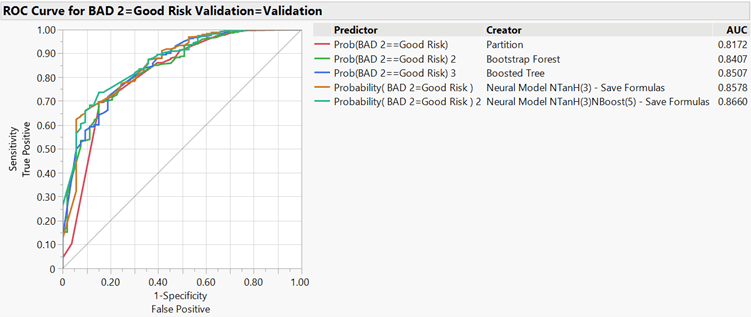
Combined ROC Curves: Related to the AUC discussion in the previous subsection, the receiver operating characteristic (ROC) curves diagram (Figure 2) shows that the boosted neural network was the most successful model for correctly classifying a good risk compared to randomly classifying a risk as good based on the outcome of a coin toss (the coin toss is represented by the diagonal gray line). A noteworthy observation of the curves in the ROC curve diagram is that although the boosted tree performed third best with respect to the overall AUC, it performed with less volatility from (0.2,0.7) as the curve approached (1,1) compared to the neural network and boosted neural network models.

Figure 2: Combined ROC Curves

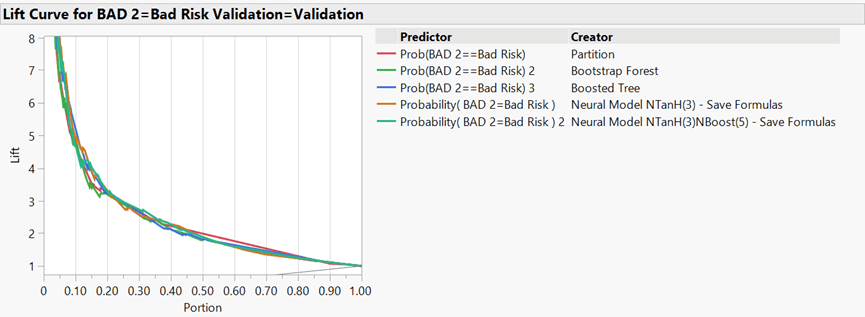
Combined Lift Curves: The combined lift curves (Figure 3) show that each model performed comparably. Each model began with a lift of approximately 8 and fell to 1 as the portion of the data increased. Each model was twice as accurate at predicting a good risk, compared to a coin toss, through approximately the first 45% of the data. Each model performed comparably with respect to the lift curves, and the lift curves behaved appropriately such that each curve began with a large lift value in the top-left corner and fell to 1 in the bottom-right corner. While the overlapping lines did moderately obfuscate the interpretability of each model individually, the boosted tree appeared to follow a less volatile curve than the neural network and boosted neural network models.

Figure 3: Combined Lift Curves

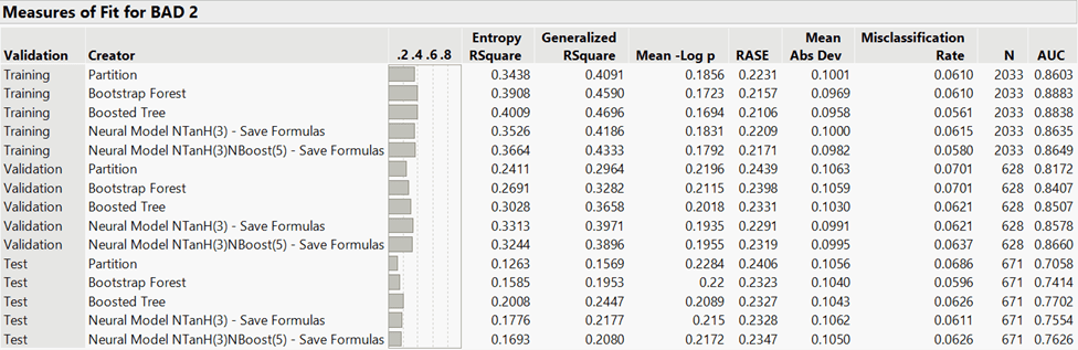
Combined Measures of Fit: The combined measures of fit diagram (Figure 4) shows the misclassification rates of the training, validation, and test sets of each model. Note that each error rate in Figure 1 was rounded based on the misclassification rate of the validation set of the respective model in Figure 4. While the validation set was used for comparative modeling, the misclassification rate and AUC of the test set of each model should be compared to that of the validation set of each respective model to determine how well each model can be expected to perform when each model is introduced to new data. As shown in Figure 4, the boosted tree and the neural network both had a misclassification rate of 6.21%, followed by the boosted neural network at 6.37%. It is important to note that the naïve misclassification rate was found to be 8% by calculating the percentage of total good risks from the total risks (BAD response variable) from the adjusted dataset and that not one model had a misclassification rate that was higher than 8%.

Figure 4: Combined Measures of Fit

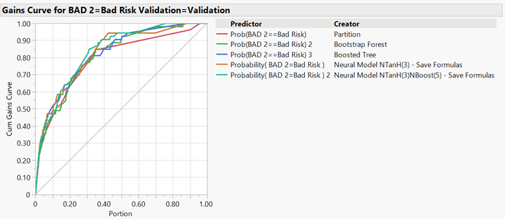
Combined Cumulative Gains Curves: The cumulative gains curve (Figure 5) shows the percentage of the total population of good risks (y-axis) when only some percentage of the population (x-axis) is considered. The gray diagonal line represents a randomly considered risk. For each model, approximately 70% of the good risks were considered once only 25% of the risks were considered. While each model performed approximately equally with respect to the cumulative gains curve up through 25% of the dataset, the first model to capture the total population was the boosted neural network at 75% of the population, followed approximately equally by the boosted tree, bootstrap forest, and neural network models at approximately 85%.

Figure 5: Combined Cumulative Gains Curves

Conclusion: The purpose of this study was to perform comparative predictive modeling to determine the best model to use to predict whether a consumer is a good risk for an HEL. Based on the comparative analysis, the boosted forest model either equally performed or outperformed the other models in each metric but the AUC and the cumulative gains curve. however, as shown in Figure 4, the difference between the AUC of the validation set and the AUC of the test set of the boosted forest model was 0.0805, or 8.05%, which was the smallest difference between the validation set AUC and the test set AUC among the models.

Assuming that the best model is the one that can be used to predict whether a consumer is a good risk for an HEL while also prioritizing risk aversion by avoiding identifying bad risks as good risks, which could expose the lender to loan defaults, as much as possible while also identifying as many good risks as possible, the boosted forest model is the best predictive model. If the quality of the raw dataset can be improved, such as more precisely explaining the existing predictors and obtaining missing values, and/or if new data, including detailed financial data, can be collated with the existing data, an opportunity cost analysis, and ideally a more comprehensive cost-benefit analysis as well as an econometric analysis, should be performed and should accompany this study to confirm that the boosted forest model is the best model to use to predict whether a consumer is a good risk for an HEL.

References: Federal Reserve et al. (2005). Credit risk management guidance for home equity lending. https://www.federalreserve.gov/boarddocs/srletters/2005/sr0511a1.pdf