NOTE: The .xlsx file is available for download; however, the data was prepared and analyzed in JMP Student Edition 18.
NOTE: Directly below this note is the data dictionary that I prepared.
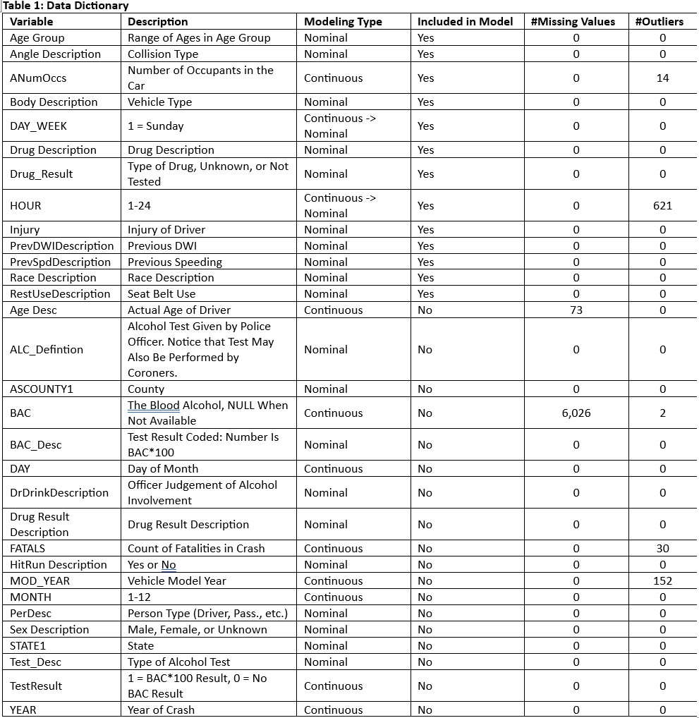
Table 1: Data Dictionary
Introduction and Business Understanding: According to the National Highway Transportation Safety Administration (NHTSA) (2025), the Fatality Analysis Reporting System (FARS) “…contains data on a census of fatal motor vehicle traffic crashes within the 50 states, the District of Columbia, and Puerto Rico.” Furthermore, for a fatal motor vehicle traffic crash to be recorded in FARS, NHTSA (2025) requires that “…a crash must involve a motor vehicle traveling on a trafficway customarily open to the public and must result in the death of a vehicle occupant or a nonoccupant within 30 days of the crash.” Recorded in the data set are data regarding blood alcohol content (BAC). Not all motor vehicle accidents result in BAC tests. The purpose of this study was to analyze the data set and to perform predictive modeling to reliably estimate the percentage of fatal crashes that involved alcohol consumption such that the BAC of the driver was greater than or equal to 0.08%. An area under the curve (AUC) of less than 80% and an overall error rate (misclassification rate) of greater than 22% were established as success/failure thresholds for this study.
Data Understanding and Preparation: The FARS raw data set contained 31 variables, of which 10 were a continuous modeling type and 21 were a nominal modeling type, and 92,824 records for fatal crashes from the years 2005 through 2013 and 2016 but not from years 2014 or 2015. The columns “PerDesc,” “Drug Result Description,” and “Test_Desc” contained only one value and were therefore excluded. Due to missing values and outliers, which will be discussed later, approximately 7.4% of the raw data was excluded from analysis. After screening the data, partitioning of the data was done. Then, the modeling type of each predictor variable was assessed to determine whether a change to the automatic modeling type was warranted. Next, A “DWI” column was created, and each predictor variable was fit against “DWI” to determine the best variables to use to predict DWI. The selected predictor variables that were of nominal modeling type were then binned either by grouping closely equal percents of factor. Additional data preparation steps are discussed in the next six subsections.
Missing Values and Outliers: Upon screening the data for missing values, it was found that there were 73 missing values in the “Age Desc” column and 6,026 missing values in the “BAC” column. After excluding the missing values, 6,091 records from the data set were excluded, indicating that 8 records shared both missing values. There was a new total of 86,733 records remaining in the data set. Upon further screening the data for outliers, it was found that outliers existed in the following counts and columns: 152 for “MOD_YEAR,” 14 for “ANumOccs,” 621 for “HOUR,” 30 for “FATALS,” and 2 for “BAC,” for a total count of 819 outliers. After excluding these records and scanning again for outliers, it was found that no outliers remained. The new total excluded count was 6,905 records for a new total of 85,919 remaining records from the previous 86,733 remaining records.
Partitioning the Data: After the screening was completed, partitioning of the data was done to create a training set (65%; 55,847 records), a validation set (20%; 17,184 records), and a test set (15%; 12,888 records).
Modeling Type: The auto-assigned modeling types were mostly appropriate but for the “HOUR” and “DAY_WEEK” predictor variables, which had to be changed to nominal for practical-use purposes.
Creation of the Response Variable “DWI”: After partitioning the data and reviewing the modeling types, the response variable “DWI” column was created by using a conditional formula to return a value of 0 if the value in the “BAC” column of a record was less than 0.08 or to return a value of 1 if the value was equal to or greater than 0.08.
Selection of Best Predictor Variables: After creating the “DWI” column, selection of best predictor variables was done by fitting “DWI” by each predictor variable and evaluating both the statistical and practical significances of each variable. The selected best predictor variables have “Yes” in the “Included in Model” column in Table 1. These 13 variables were sorted to the top of the table for ease of reference.
Binning: Binning was then done to the selected best predictor variables in the training set; binning decisions in the training set do not affect the validation set. Only the 11 nominal selected best predictor variables were binned.
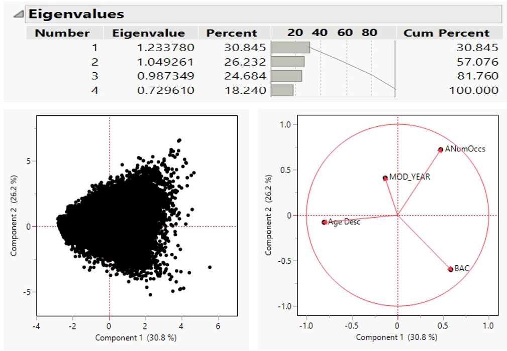
Principal Components (Loading Chart): The continuous variables “Age Desc,” “MOD_YEAR,” “ANumOccs,” and “BAC” were used to generate the Principal Components on Correlations (see Figure 1). The first two principal components explained approximately 57% of the variance within the data (see Figure 1). According to the loading chart, “ANumOccs” loaded positively with both Component 1 and 2, “MOD_YEAR” loaded negatively with Component 1 but positively with Component 2, “Age Desc” loaded negatively with both Component 1 and 2, and “BAC” loaded positively with Component 1 but negatively with Component 2. None of the variables had a strong correlation with any other.
Figure 1: Eigenvalues and PCA
Model Understanding: Because the purpose of this study was to reliably estimate the percentage of fatal crashes that involved alcohol consumption such that the BAC of the driver was greater than or equal to 0.08%, binary categorical outcomes of either 1, representing yes, or 0, representing no, were predicted. Based on the purpose of this study, a logistic regression model (LRM) was the most appropriate model to reliably classify a new observation into one of the binary categorical classes. In this case, an observation was either coded to belong to either the class of drivers with a BAC greater than or equal to 0.08% or not. A cutoff value of 0.5, or 50%, was used.
An LRM uses the logit, or the logarithm of the odds (log(odds)), to determine the relationship between the logit and the predictors and models the logit as a linear function of the predictors. Once the logit is computed, the logit can be converted to the propensity that the driver will have a BAC greater than or equal to 0.08% by Equation 1:

where Lini(1) is the logit value of observation i, calculated in JMP. If
was greater than or equal to the cutoff value, then the observation was classified as 1, meaning that the observation had the propensity of belonging to the class of drivers with a BAC greater than or equal to 0.08%. The efficacy of the LRM model was assessed by interpreting the confusion matrix (Figure 3), the receiver operating characteristic (ROC) (Figure 4), and the lift curve (Figure 5) of the validation set.
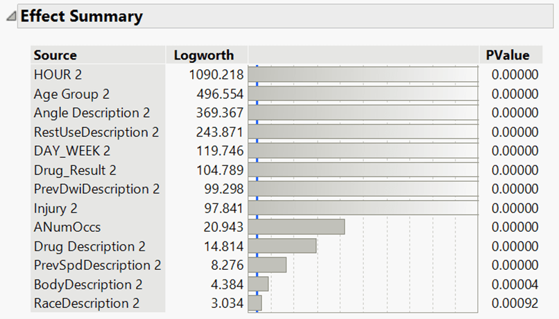
Model Analysis: Upon running the LRM, it was found that the top predictor was “HOUR,” with the greatest logworth (the negative logarithm of base 10 of the p-value) of 1,090.218, indicating that “HOUR” had the smallest p-value out of the predictors. The predictor “Race Description” had the least logworth of 3.034. The remaining 11 predictors had a logworth between these logworths. See Figure 2 (Effect Summary) for more details. At 5 decimal places, the best 11 predictors all returned a p-value of 0.0000, making it difficult to determine the strength of each predictor relative to the logit. The logworth provides a representative value of the p-value, making it easier to better understand the relative strength of the predictors. It is important to note that logworth is specific to JMP and that more information can be found in the JMP User Community discussions (see References).
Figure 2: Effect Summary
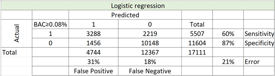
Confusion Matrix of Validation Set: A confusion matrix of the validation set was then analyzed to determine the overall error rate, sensitivity, specificity, false positive, and false negative percentages of the validation set (Figure 3). The overall error rate, or the misclassification rate, was 21.48%. The sensitivity and specificity indicate the true positive and negative percentages, and the false positive and false negative indicate the percentages of the prediction that are incorrect.
The 60% sensitivity and 87% specificity indicated the ability of the model to correctly classify an observation in each class (either 1 or 0 for the purpose of this study). This means that the model correctly classified 60% of the true 1 class and 87% of the true 0 class.
The 31% false positive and 18% false negative values indicated the failure of the model to correctly classify an observation. This means that the model proportionally incorrectly predicted 31% of class 1 and 17% of the class 0.
Figure 3: Logistic Regression Confusion Matrix
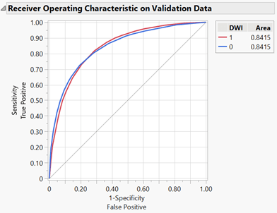
ROC Curve of Validation Set: The sensitivity and specificity were then plotted on a ROC curve (Figure 4), where the true positive is plotted on the y-axis and the false positive is plotted on the x-axis. The solid diagonal line represents a 0.5 probability, or 50% probability, of randomly classifying an observation. An AUC greater than 0.5 indicates the probability that a randomly selected observation will be classified correctly. The AUC of the ROC curve of the validation set was 0.8415, or 84.15%.
Figure 4: ROC Curve
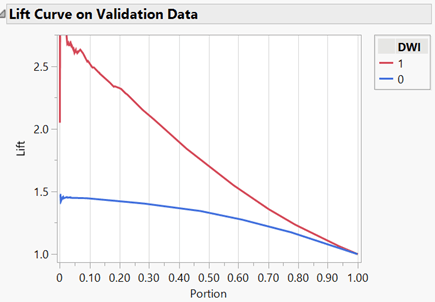
Lift Curve of Validation Set: A lift curve shows the ratio of the cumulative correct classification of the response variable over the cumulative classification by randomly classifying the response variable (e.g., flipping a coin). When there is high lift when only a small portion of the data is considered and when the curve approaches a lift of 1 as the portion of the data approaches 1.00, or 100%, along the x-axis, the model exhibits a strong predictive ratio of the response variable. This behavior was observed (see Figure 5). This indicated that the model better predicted a correct classification of an observation than correctly classifying an observation at random. For example, when only 30% of the data was considered, the model correctly classified the response variable twice as well than if the response variable were randomly classified.
Figure 5: Lift Curve
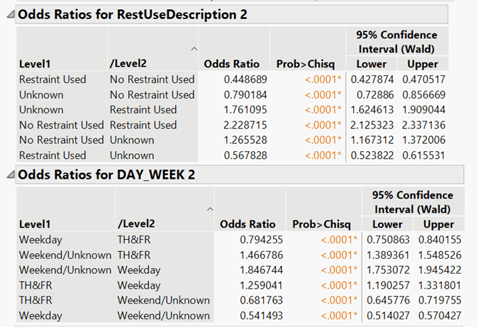
Odds Ratio: The odds ratios for the restraint system used by the drivers and the days of the week were assessed (see Figure 6). The most notable ratio of the restraint system used was no restraint use to that of restraint use. The odds of a driver in a fatal crash not using a restraint system was approximately 2.23 times the odds of a driver using a restraint system. The odds of a fatal crash occurring on a weekend was approximately 1.85 times the odds of a fatal crash occurring on a weekday.
Figure 6: Odds Ratios
Conclusion: The AUC and overall error rates were 84.15% and 21.48%, respectively. The lift curve also behaved as intended. Thus, this model was valid. The results of the specificity and false negative percentages of the confusion matrix were good, but the sensitivity and false positive percentages were less than favorable. To potentially improve the model, possibly imputing missing or unknown values, obtaining and including the missing and unknown values, creating and adding interaction predictors, reducing the number of predictors for parsimony, and/or adjusting the cutoff value could be attempted. Depending on the tolerance for a marginally increased error rate (21.85%), a marginally lower AUC (83.67%), and a decently higher sensitivity (64.4%) with a slightly increased false positive percentage (33.4%) by lowering the cutoff value to 47% and using only “HOUR,” “Age Group,” “Angle Description,” “RestUseDescription,” “DAY_WEEK,” “Drug_Result,” and “Injury” as predictors, ordered by logworth descending, a more parsimonious model can be achieved.
References:
hartpjb. (2022, September 13). What does logWorth measure that is not included in the anova table of a fit model analysis? [JMP User Community Discussion form]. https://community.jmp.com/t5/Discussions/What-does-logWorth-measure-that-is-not-included-in-the-anova/td-p/544036
National Highway Traffic Safety Administration (NHTSA). (2025, March 18). Fatality analysis reporting system. U.S. Department of Transportation. https://www.nhtsa.gov/crash-data-systems/fatality-analysis-reporting-system
rlw268. (2020, September 15). Effect summary and the logworth with p-value of 0???? [JMP User Community Discussion forum]. https://community.jmp.com/t5/Discussions/Effect-Summary-and-the-Logworth-with-p-value-of-0/td-p/307974
